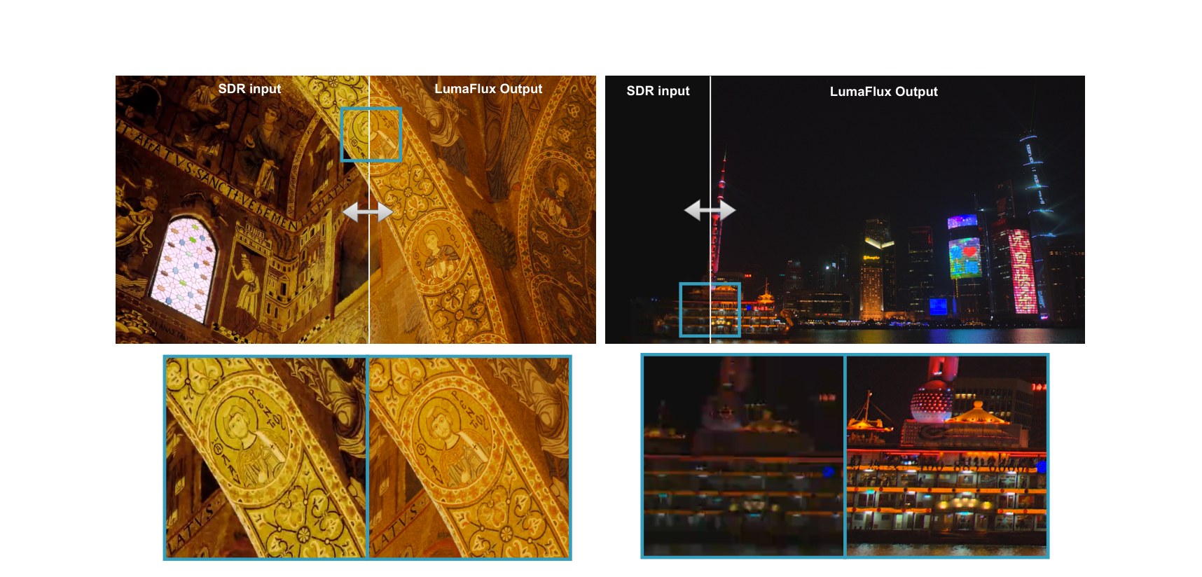
Thesis. SDR→HDR conversion fails in two different ways: regression models can't hallucinate the structure that tone mapping destroyed, and generative models hallucinate too much because nothing anchors them to physical luminance. The fix is to keep a pretrained diffusion transformer entirely frozen — it already knows what images look like — and inject only the physics it is missing.
Main technical point. Four zero-initialized modules steer the frozen backbone: gated low-rank attention updates driven by luminance/gradient/frequency cues (PGA), FiLM conditioning on SigLIP semantics (PCM), a timestep- and layer-gated residual coupler, and a monotone rational-quadratic spline that performs the actual dynamic-range expansion after the VAE decoder.
Practical implication. Prompt-free, parameter-efficient ITM that converts real-world 8-bit BT.709 video to 10-bit PQ/BT.2020, outperforming CNN and diffusion baselines by up to +1.6 dB PSNR and −0.8 ΔEITP — trained in ≈2 days on 4× H200 (≈190 GPU-hours) because only the adapters update.
Background
Why Inverse Tone Mapping Is Genuinely Hard
An SDR frame is not a smaller HDR frame — it is the output of a lossy, device-dependent chain1:
\[ x_{\mathrm{sdr}} \;=\; \Gamma^{709}_{\mathrm{OETF}}\!\Big( M_{2020\rightarrow709}\,\Gamma^{2020}_{\mathrm{EOTF}}\big(x_{\mathrm{hdr}}\big)/L_{\max} \Big) + \epsilon . \]
The SDR formation model: tone curve ∘ gamut compression ∘ quantization/codec noise ε.
Three different kinds of information die in that chain. Specular highlights above ~100 nits are clipped or rolled off — a many-to-one mapping with no unique inverse. Wide-gamut colors outside BT.709 are projected onto the gamut boundary, which is why up-converted sunsets and neon signs look desaturated. And 8-bit quantization plus codec compression erase the low-amplitude texture that would have disambiguated the rest.
Classical operators (Reinhard, the BT.2446 family) invert only the global curve: content-blind, prone to over-brightening flat regions and clipping highlights. Supervised CNNs (HDRTVNet++, HDCFM, Deep SR-ITM) regress the mapping from paired data but overfit the specific tone-mapper and codec mix they were trained on. Recent diffusion approaches (LEDiff, PromptIR) bring generative priors but retrain large backbones or depend on text prompts — and a caption is a terrible place to encode "this pixel was 800 nits."
Approach
Borrow the Prior, Don't Retrain It
The starting observation is that large diffusion transformers are surprisingly tone-invariant. For any monotone tone map \(\phi\), the direction of the learned velocity field is approximately preserved:
\[ \operatorname{dir} f_\theta\big(\mathcal{E}(\phi(x))_t, t\big) \;\approx\; \operatorname{dir} f_\theta\big(\mathcal{E}(x)_t, t\big), \]
i.e., the model encodes edges, textures, and cross-channel correlations — relative structure — rather than absolute luminance. That is exactly the information ITM needs to hallucinate plausible highlight detail, and it survives tone mapping. So instead of fine-tuning (which overfits small HDR corpora and hallucinates texture), LumaFlux freezes every backbone weight and inserts adapters that supply what the prior lacks: physical luminance.
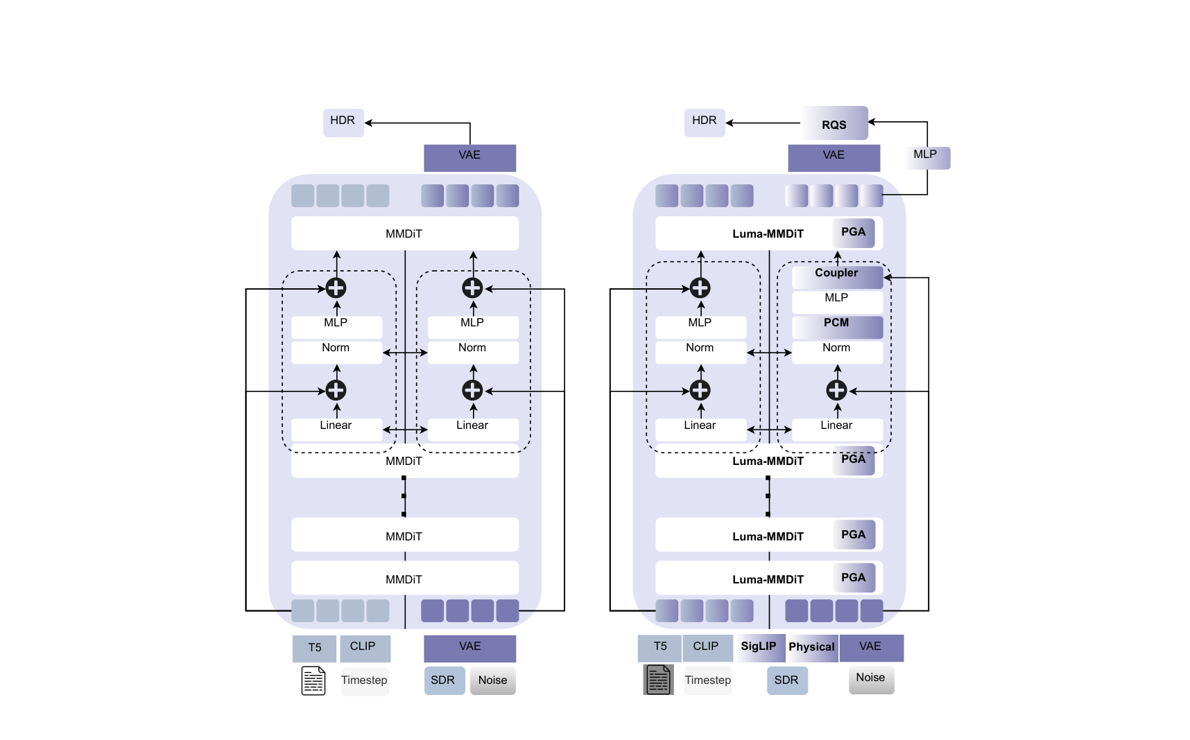
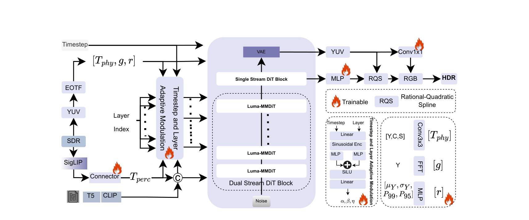
Everything trainable is scheduled by a shared conditioner \(\Psi(t,\ell)\) over flow time \(t\) and block index \(\ell\), emitting per-block gains \((\alpha^{t,\ell}_{\mathrm{pga}}, \beta^{t,\ell}_{\mathrm{pga}}, \alpha^{t,\ell}_{\mathrm{pcm}}, \beta^{t,\ell}_{\mathrm{pcm}}, n^{t,\ell}_{\mathrm{spec}}, \lambda^{\ell}_t)\). Early layers and large \(t\) get strong global tone corrections; late layers and small \(t\) focus on highlight micro-structure. Every adapter is zero-initialized, so at step 0 the system is the pretrained model.
Method
PGA: Attention That Knows Where the Light Was
From the linearized input we build a physical descriptor map — luminance, log-gradient magnitude, saturation — plus global statistics \(s_g = [\mu_Y, \sigma_Y, p_{95}, p_{99}]\) and a \(K\)-band FFT energy vector \(r\) of the luminance spectrum:
\[ T_{\mathrm{phys}} = \mathrm{Conv}_{3\times3}\big([\,Y,\ \log(1+|\nabla Y|),\ \mathrm{sat}\,]\big), \qquad g = \mathrm{MLP}_g(s_g). \]
Physically-Guided Adaptation then perturbs each frozen value projection \(W_V^{(0)}\) with a gated low-rank residual. A plain LoRA update \(R^{\mathrm{base}}_v = A_v B_v\) would apply everywhere uniformly; PGA modulates it per token and per attention head by the physical cues, and per head by spectral energy:
\[ G_{\mathrm{phys}} = \mathrm{Diag}\big(\sigma(P_v[T_{\mathrm{phys}} \| g])\big), \qquad g_{\mathrm{FFT}} = \mathrm{softplus}(W_r r), \]
\[ R^{t,\ell}_v = \big(\alpha^{t,\ell}_{\mathrm{pga}} R^{\mathrm{base}}_v + \beta^{t,\ell}_{\mathrm{pga}} I\big)\, G_{\mathrm{phys}} \big(I + n^{t,\ell}_{\mathrm{spec}}\,\mathrm{Diag}(g_{\mathrm{FFT}})\big), \qquad W_V \leftarrow W_V^{(0)} + R^{t,\ell}_v . \]
The effect is surgical: highlight and high-frequency pathways strengthen only where the scene contains highlights and texture, so flat regions are never over-expanded and highlight roll-off stays physically consistent. In the ablation, PGA alone is worth +1.8 dB over Flux + LoRA, and spectral gating adds measurable HDR-VDP3 on top.
Method
PCM and the HDR Residual Coupler
Not all tone-mapping damage is photometric. Hue drift, oversaturation, and texture inconsistency are perceptual failures — the loss of semantic and chromatic coherence across regions. Perceptual Cross-Modulation conditions the hidden states on frozen SigLIP embeddings through a learned connector \(C_{\mathrm{perc}}\), as FiLM2:
\[ [\gamma^{t,\ell}, \zeta^{t,\ell}] = \alpha^{t,\ell}_{\mathrm{pcm}}\,\mathrm{MLP}\big(C_{\mathrm{perc}}(T_{\mathrm{perc}})\big) + \beta^{t,\ell}_{\mathrm{pcm}}, \qquad \mathrm{PCM}(h_\ell) = \gamma^{t,\ell} \odot \mathrm{LN}(h_\ell) + \zeta^{t,\ell}. \]
Because the SigLIP image tokens also join the (otherwise learned, prompt-free) context sequence, the model gets semantics without a single caption — no T5, no CLIP text tower, no semantic drift from a wrong prompt.
Finally, the HDR Residual Coupler re-injects both streams into each block's residual path with a time- and layer-dependent gate:
\[ z^{\ell}_{\mathrm{out}} = z^{\ell}_{\mathrm{res}} + \lambda^{\ell}_t\big(W_p T_{\mathrm{phys}} + W_c\, C_{\mathrm{perc}}(T_{\mathrm{perc}})\big). \]
\(\lambda^\ell_t\) decays as \(t \to 0\): early steps prioritize global tone recovery (contrast, exposure alignment), late steps refine local highlight roll-off. It behaves like classifier-free guidance, but implemented as additive couplings inside the latent manifold rather than extrapolation off of it.
Method
The RQS Tone Field: Don't Trust an SDR-Trained VAE
Here is the failure mode nobody escapes by training adapters alone: the Flux VAE was trained on 8-bit imagery. Its decoder is calibrated to the SDR luminance manifold, so asking it to emit HDR directly invites banding, highlight clipping, and gamut misplacement. Fine-tuning the VAE is expensive and risks destroying the prior. LumaFlux instead appends a tiny, provably monotone tone expander: a rational-quadratic spline (Durkan et al.'s neural-spline construction) whose parameters \((\xi, \eta, s)\) are predicted per frame from the final latent:
\[ \hat{Y} = \mathrm{RQS}\big(Y_{\mathrm{out}};\, \xi, \eta, s\big), \qquad \hat{x}_{\mathrm{hdr}} = M_{\mathrm{YUV}\rightarrow\mathrm{RGB}}\big([\hat{Y}, \hat{U}, \hat{V}]\big)_{\mathrm{PQ,\,BT.2020}} . \]
Monotonicity guarantees no tone inversions; differentiability and bounded derivatives give smooth highlight knees without banding; and with \(K \geq 6\) bins an RQS can uniformly approximate any reasonable monotone tone map — so the frozen DiT supplies structure while the spline supplies calibrated luminance. The ablation makes the case crisply: replacing the spline with a linear tone head hurts (over-contrast, banding), while the monotone spline is the single biggest ΔEITP and HDR-LPIPS improvement in the stack.
The full inference path, prompt-free, 40 ODE steps:
- Featurize. Linearize the SDR frame; compute \(T_{\mathrm{phys}}, g, r\) and SigLIP tokens \(T_{\mathrm{perc}}\); encode \(z = \mathcal{E}_{\mathrm{VAE}}(x_{\mathrm{sdr}})\).
- Integrate. For each step \(t: 1 \to 0\) and block \(\ell\): evaluate \(\Psi(t,\ell)\), apply PGA to \(W_V\), FiLM the normalized activations, couple the residual, and take a frozen-backbone Euler step.
- Decode + expand. Decode with the frozen VAE, convert to YUV (BT.2020), apply the predicted RQS to luma and 1×1 refinements to chroma, and re-encode as PQ/BT.2020.
Data & Benchmark
A Corpus That Matches Reality, and Luma-Eval
Models trained on a single tone-mapper memorize its curve. We curate the first large-scale real-world SDR–HDR corpus by unifying HIDROVQA (411 professional HDR videos), CHUG (428 crowdsourced UGC HDR videos), and LIVE-TMHDR (40 studio videos with expert-graded SDR) into PQ/BT.2020 at a 1,000-nit mastering peak, then pairing every HDR frame with SDR variants from a composite degradation chain:
\[ x_{\mathrm{sdr}} = Q_{\mathrm{codec}} \circ M_{2020\rightarrow709} \circ T_{\mathrm{MO}}(x_{\mathrm{pq}};\theta_{\mathrm{tone}}), \]
with eight tone-mapping operators (OCIOv2-style, BT.2446a, BT.2446c+GM, hard-clip+GM, Reinhard, a YouTube-LogC-style curve, BT.2390-EETF+GM, gamma-clip) crossed with x264 at CRF 23/31/39 — ≈318k pairs, sampled 1:1 PGC:UGC during training. Luma-Eval holds out 20 sources (10 PGC, 10 UGC) and evaluates under both expert-graded and degradation-heavy SDR, alongside HDRTV1K and HDRTV4K re-normalized to the same standard.
Results
What the Numbers Say
Across HDRTV1K, HDRTV4K, and Luma-Eval, LumaFlux leads on pixel fidelity and perceptual color simultaneously — the combination prior methods trade against each other. On Luma-Eval:
| Method | PSNR ↑ | SSIM ↑ | HDR-VDP3 ↑ | ΔEITP ↓ |
|---|---|---|---|---|
| HDRTVNet++ | 36.54 | 0.901 | 8.22 | 7.35 |
| HDCFM | 36.78 | 0.915 | 8.29 | 7.20 |
| PromptIR | 34.12 | 0.913 | 8.88 | 6.82 |
| LEDiff | 31.73 | 0.859 | 5.12 | 9.85 |
| FlashVSR | 34.80 | 0.857 | 5.84 | 6.23 |
| LumaFlux (ours) | 36.92 | 0.938 | 8.91 | 5.67 |
Generalization across degradations is the more telling number: per-TMO breakdowns stay within a ≈3 dB band from the easiest (BT.2446c+GM, 38.31 dB) to the hardest (YouTube-LogC, 35.12 dB) SDR styles, including expert-graded SDR (37.11 dB) that no synthetic TMO mimics. A 10-expert user study on a UHD-HDR monitor agrees: LumaFlux scores highest on brightness realism (3.8), color naturalness (4.5), and overall HDR quality (4.2 MOS), with raters specifically noting restored highlight detail without midtone over-amplification.
What each piece buys (ablation, Luma-Eval)
| Variant | PSNR ↑ | ΔEITP ↓ | HDR-VDP3 ↑ | HDR-LPIPS ↓ |
|---|---|---|---|---|
| Flux + LoRA only | 33.42 | 8.58 | 7.82 | 0.136 |
| + PGA (no spectral) | 34.94 | 7.62 | 8.18 | 0.122 |
| + PGA (spectral gating) | 35.18 | 7.31 | 8.29 | 0.116 |
| + PCM (SigLIP FiLM) | 35.89 | 6.78 | 8.46 | 0.107 |
| + RQS (linear) | 35.72 | 6.85 | 8.41 | 0.108 |
| + RQS (monotone spline) | 35.98 | 6.09 | 8.61 | 0.087 |
Code
Implementation
A complete from-scratch implementation — data curation, training (HuggingFace
diffusers/accelerate with
trackio tracking), prompt-free inference, PU21/ΔEITP evaluation,
and a Gradio demo — lives at
github.com/shreshthsaini/LumaFlux. The core loop:
def lumaflux_convert(model, x_sdr, num_steps=40):
    # physical + perceptual conditioning (prompt-free)
    cond = model.prepare_condition(x_sdr)        # T_phys, g, r, SigLIP tokens
    z = pack_latents(model.encode_image(x_sdr))  # z_1 = E_VAE(x_sdr)

    ts = torch.linspace(1.0, 0.0, num_steps + 1)
    for i in range(num_steps):                   # frozen-backbone Euler ODE
        t = ts[i].expand(z.shape[0])
        v = model.velocity(z, t, cond)           # PGA + PCM + coupler inside
        z = z + (ts[i + 1] - ts[i]) * v

    return model.decode_hdr(z)                   # frozen VAE -> RQS tone field
Practical notes from the implementation:
- Zero-init everything. All adapter paths (low-rank up-projections, FiLM MLPs, coupler projections, spline head) start at exactly zero contribution — the wrapped transformer reproduces the frozen backbone bit-for-bit at step 0, which makes early training loss identical to the prior's and prevents collapse.
- Identity-init the spline. Uniform knots need derivative bias \( \mathrm{softplus}^{-1}(1) \approx 0.541\), not zero — otherwise the "identity" spline bends mid-bin.
- Mind pow() gradients. PQ and OETF curves have exponents < 1; their gradients are NaN at exactly 0. Clamp to tiny positives (value impact < 1e-18 linear) or one black pixel poisons the run.
- Train on the bridge you sample. We flow-match the noisy linear bridge between SDR and HDR latents, so inference can start at \(z_1 = \mathcal{E}(x_{\mathrm{sdr}})\) exactly as trained — no train/test trajectory mismatch.
References
- Saini et al., LumaFlux: Lifting 8-Bit Worlds to HDR Reality with Physically-Guided Diffusion Transformers, 2026.
- Black Forest Labs, Flux.1, 2024.
- Durkan et al., Neural Spline Flows, NeurIPS 2019.
- Perez et al., FiLM: Visual Reasoning with a General Conditioning Layer, AAAI 2018.
- Zhai et al., Sigmoid Loss for Language Image Pre-Training (SigLIP), ICCV 2023.
- Chen et al., A New Journey from SDRTV to HDRTV (HDRTV1K), ICCV 2021.
- Guo et al., Learning a Practical SDR-to-HDRTV Up-Conversion (HDRTV4K), CVPR 2023.
- Venkataramanan and Bovik, Subjective Quality Assessment of Compressed Tone-Mapped HDR Videos (LIVE-TMHDR), IEEE TIP 2024.
- Saini et al., HIDRO-VQA: High Dynamic Range Oracle for Video Quality Assessment, WACV 2024.
- Saini et al., CHUG: Crowdsourced User-Generated HDR Video Quality Dataset, ICIP 2025.
- Mantiuk et al., HDR-VDP-3, 2023.
- Wang et al., LEDiff: Latent Exposure Diffusion for HDR Generation, CVPR 2025.